Types of Data Analytics Charts and How They Improve Your Product (+ Blind Spots)

Data analytics charts play a key role in tracking whether new features are landing, where users drop off, and which cohorts are quietly disengaging before anyone on the customer success team notices.

But knowing which visual representation of that data to trust, and when, makes a huge difference.

Most product teams pick chart types by habit: bar chart for comparisons, line chart for trends, funnel when something looks broken. That instinct is mostly right, but it breaks down the moment the data underneath changes.

This guide covers ten types of data analytics charts you’ll find in most product analytics platforms.

Bar data analytics charts

Bar charts are the most widely used data visualization format in product analytics. They represent data using rectangular bars whose lengths correspond proportionally to the values they show, making it easy to compare categories at a glance. The logic is simple: longer bar means larger value, and that visual representation is one that most readers parse without any explanation.

Types of bar charts

• Standard bar chart: One horizontal bar per category, ideal for comparing individual values cleanly across a small number of groups. It’s the most direct tool for answering “which of these is biggest?” without adding visual complexity.
• Grouped bar chart: Displays multiple sub-groups side by side within each category. Useful when you’re comparing, for example, how feature engagement differs between free and paid users across the same time period, rather than just comparing one number per category.
• Stacked bar chart: Stacks sub-groups within a single bar to show both the total and its composition. These are good for visualizing how multiple categories contribute to a whole, though it gets hard to read when you have more than four or five sub-groups sharing the same bar.

When to use bar charts

Bar charts work best when you’re comparing values across different categories at a single point in time. Ranking features by adoption rate, comparing support ticket volume by type, or seeing which user segments are most active are all natural fits. For categorical data where order matters (like ranking), it’s worth sorting bars from highest to lowest so the comparison lands faster for anyone reading quickly.

Remember to always start the axis at zero. A bar chart with a truncated y-axis makes a small difference look like a dramatic gap, which leads to the wrong decisions in planning meetings.

Bar chart example

One way to use bar charts is to compare feature adoption across user segments in a single view. Seeing which features are driving engagement among paid users versus trial users tells you immediately where to focus onboarding guidance in the next sprint, without needing to cross-reference multiple reports.

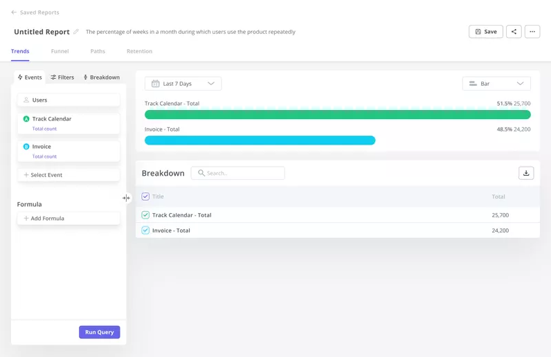
The blind spot: Bar charts are snapshots. They tell you where things stand today, but they can’t show whether the situation is improving or declining over time. If the question you’re trying to answer involves direction or trend, you need a line chart.

Column data analytics charts

Column charts display data in vertical bars, making them naturally suited for time-series data where the x-axis runs from left to right. They carry the same core logic as bar charts but the vertical orientation makes it easier to read data across time intervals, which is why they show up constantly in user activity trend reports.

Types of column charts

• Clustered column chart: Groups multiple data series side by side within each category. Works well when you need to compare how different segments perform at the same point in time, and it handles medium-sized datasets without becoming visually cluttered.
• Stacked column chart: Stacks data series vertically within each column to show both the total value and each sub-group’s contribution. Useful when multiple categories add up to a meaningful total, like daily active users broken down by plan type.

When to use column charts

Column charts are strong for comparing values across ordered time intervals: weeks, months, or quarters. They communicate ranking and trend direction at the same time, which makes them a reliable choice when you need stakeholders to quickly understand both the absolute numbers and the direction of movement.

Column chart example

A stacked column chart can help you track daily active users by plan type over time. When a spike in engagement appears, the stacked format immediately separates whether that spike came from paid accounts or trial users, so you don’t misread a trial-driven bump as genuine retention growth.

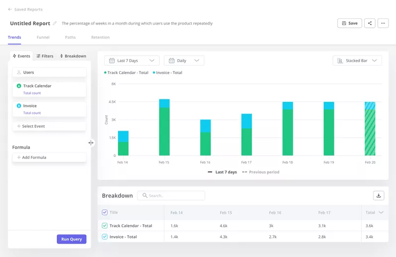
The blind spot: Column charts compress badly when you have too many time periods. Monthly data across three years becomes a wall of thin columns where individual values are unreadable. If you need to show more than 20 time periods, switch to a line chart, which handles density far better.

Line data analytics charts

Line charts connect individual data points with a continuous line, making them the standard format for showing how a metric changes over time. They’re particularly strong at highlighting trend direction, identifying turning points in data, and comparing the trajectory of multiple variables on the same axis.

Types of line graphs

• Basic line chart: A single line tracking one metric over time. Clean and readable, ideal when you’re monitoring one key data point like weekly signups or monthly revenue without adding comparison complexity.
• Multiline chart: Multiple lines on the same chart, each representing a different variable or segment. Useful for comparing how different groups, like desktop and mobile users, engage with a feature across the same time period, though it gets cluttered beyond four or five lines.

When to use line charts

Line charts are the right tool for tracking trends over continuous time, spotting seasonal patterns, and comparing segment trajectories in parallel. They also work well for visualizing cumulative effects, like a running total of users who have completed activation since a product launch. One rule that matters: line charts imply continuity between data points, so if your data has meaningful gaps, the line creates a false impression of smoothness where none exists.

Line chart example

A multiline chart helps you track product usage by device type. Seeing mobile, desktop, and browser extension engagement plotted together over the same time period immediately tells you which platform needs prioritization in the next release cycle, without needing to run three separate reports and compare them manually.

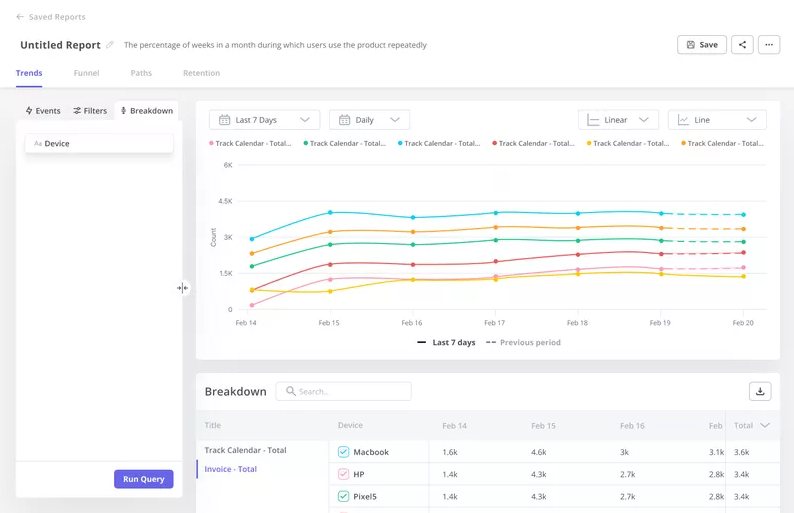
The blind spot: Beyond four or five lines, multiline charts become visual noise. Overlapping lines in similar colors are difficult to track across the chart, and the comparison you set out to make gets lost in the clutter. When you have many segments to compare, small-multiples layouts (separate mini-charts per segment) or a table will communicate more cleanly.

Funnel data analytics charts

Funnel charts show the progressive reduction of data as it moves through a sequential process. They start at 100% and narrow at each stage, giving you a clear view of where users are completing a flow versus where they’re abandoning it. In product work, funnel analysis is one of the most directly actionable chart types because it shows you the specific step where you’re losing people.

Funnel chart types

• Vertical funnel chart: Data flows top to bottom, narrowing as users progress through sequential steps. This is the most common format for onboarding flows, sales processes, and activation paths where steps must happen in a fixed order.
• Horizontal funnel chart: The same data displayed left to right. This format fits better in presentation and dashboard layouts where horizontal space is more available than vertical.

When to use funnel charts

Funnel charts are the right tool any time you need to understand how users progress through a sequential process and where the biggest drop-offs occur. They’re useful for visualizing the user journey, mapping the stages of a sales pipeline, or diagnosing activation flows where one broken step is quietly killing conversions downstream.

Funnel chart example: Finding and fixing a drop-off without engineering

When we launched our email feature, I noticed a significant drop-off in the first two steps of the activation flow. Users had been given access to the feature, but they weren’t completing domain verification, which was required before anything else could work.

The funnel data pinpointed exactly which step was losing people, so I didn’t need to guess.

“Within a few hours of seeing the chart, I built a targeting tooltip and an in-app checklist in Userpilot that walked users through domain verification step by step. The drop-off closed within days, and the entire fix happened without involving the dev team at all.”

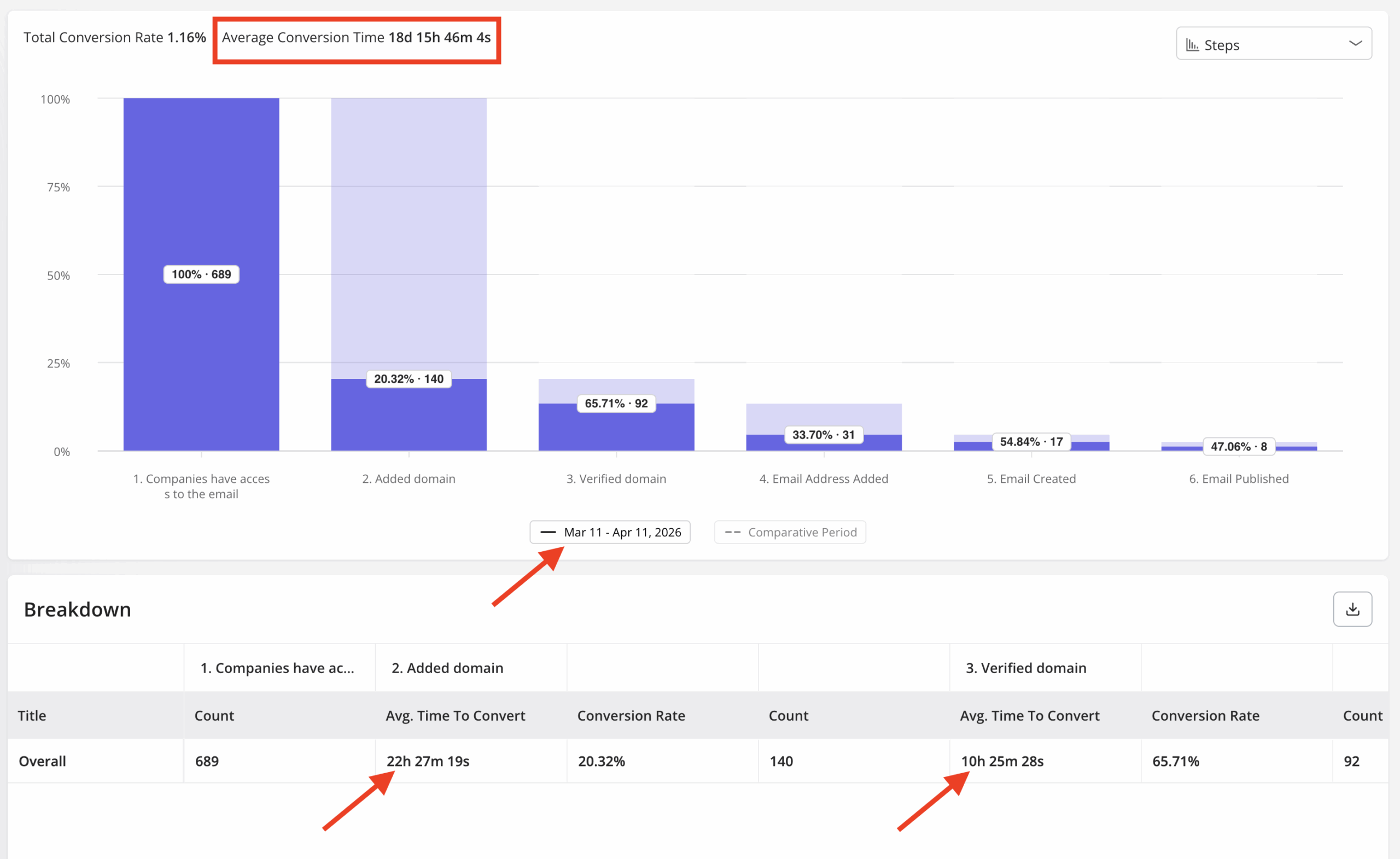
The blind spot: A funnel chart tells you exactly where users drop off, but can’t tell you why they dropped off at that step. The chart will show you that step 3 has a 60% exit rate, but without session replay or a targeted in-app survey, you’re still guessing whether users were confused, technically blocked, or simply not ready to proceed.

Pie data analytics charts

Pie charts display data as proportional slices of a circle, where each slice represents a category’s share of the whole. They’re among the most recognizable chart formats in business, which also makes them among the most frequently misused. Pie charts have a specific and narrow use case, and outside of it they consistently make data harder to interpret.

Types of pie charts

• Basic pie chart: A circular chart divided into slices that each represent a category’s proportion of the total. Works cleanly when you have a small number of categories with clearly distinct values, and you want to show part-to-whole relationships at a glance.
• Exploded pie chart: One or more slices are visually separated from the main chart body to draw attention to a specific segment. Useful when a particular category is the focus of the analysis, and you want viewers to look at it first.
• Donut chart: A pie chart variant with a hollow center. The empty space can display overall totals or a summary figure, and the ring format makes it marginally easier to compare segments than a standard pie chart because it removes the center point that distorts angle perception.

When to use pie charts

Pie charts work best when you have fewer than six or seven categories, the proportions between them are meaningfully different from one another, and you’re communicating at a single point in time rather than tracking change. They’re appropriate for showing what percentage of your users are on each pricing plan, or how revenue breaks down by product line at the end of a quarter.

Pie chart example

A great use case for pie charts is to watch feature frequency broken down by plans. This way, you can find out which type of users are more likely to engage with specific features.

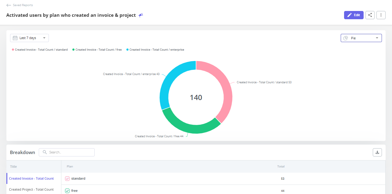
The blind spot: Human perception of angles is poor. Two slices at 23% and 27% look nearly identical in a pie chart, even though they represent a meaningful difference in a planning context. Beyond six categories, pie charts become visual noise rather than data clarity.

Heatmaps

Heatmaps use a color-coded system to represent the intensity or density of data across a surface. In product and web analytics, the surface is usually a UI screen or a web page, and the color scale shows where users are concentrating their attention and actions. Warmer colors (red, orange) indicate higher activity; cooler colors (blue, green) indicate lower activity.

The result is an immediate visual read of where a page or interface is drawing engagement and what’s being ignored, without having to parse raw event data row by row.

Types of heatmaps

• Click heatmaps: Show where users click or tap most often, making the most and least interactive elements of your UI visible without digging through event data.
• Scroll heatmaps: Show how far down a page users scroll before leaving. These reveal whether key content sits above the fold where most users reach it, or below where the majority stop.
• Move heatmaps: Track cursor movement across a page, which is a rough but useful proxy for where users are reading and considering.
• Eye tracking heatmaps: Use specialized hardware to capture actual gaze patterns, providing more precise visual attention data than cursor movement allows.
• Engagement heatmaps: Aggregate multiple behavioral signals to show which interface areas hold attention longest and generate the most sustained user engagement.

When to use heatmaps

Heatmaps are most useful for understanding how layout and design choices affect user interaction at the page or screen level. They’re strong for validating landing page designs, diagnosing navigation problems, and identifying which UI elements actually draw attention versus which ones are invisible to most users despite their prominence in the design.

Heatmap example

A practical use case is analyzing landing page click patterns to understand where visitors focus before converting. If the heatmap shows heavy clicks on a secondary navigation element instead of the primary CTA, that’s a clear signal that visitors aren’t finding what they came for, and the page hierarchy needs rethinking.

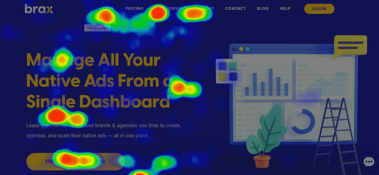
The blind spot: Heatmaps show where users click, not whether those clicks are positive signals. High click density on a “Get started” button looks promising until you realize those users are bouncing at the very next step. Always pair heatmap data with funnel analysis to understand whether the activity the heatmap reveals is leading anywhere useful.

Cohort tables

Cohort tables are one of the most powerful tools in product analytics and also among the most underused. They group users who share a common characteristic (usually their signup date or a specific action they took) and then track how that group behaves over time. The result is a matrix that shows how engagement, retention, or feature adoption evolves for a specific population across weeks or months.

Types of cohort table

• Time-based cohort table: Groups users by the period in which they took a key action, such as signing up or completing onboarding, and tracks their behavior in subsequent periods. This is the most common format for retention rate tracking because it shows you not just whether users stayed, but how each batch of users behaves compared to earlier batches.
• Behavioral cohort table: Groups users based on a specific action they took, like completing a particular onboarding step or using a certain feature, and correlates that behavior with downstream outcomes like retention or conversion.

When to use cohort tables

Use cohort tables when you need to understand whether changes you’re making are actually improving user behavior over time, not just in aggregate. Measuring the long-term impact of a new onboarding flow, tracking whether users who adopt a specific feature retain at a higher rate, or identifying which signup cohorts are churning earliest are all cases where cohort tables give you information that aggregate retention numbers hide.

Cohort table example: how ClearCalcs tracks activation by segment

ClearCalcs, a structural engineering calculation platform, used cohort analysis in Userpilot to track user activation rates at a segment level rather than as a single aggregate metric. Chris Borzillo, CEO and co-founder of ClearCalcs, separated cohorts by role, company size, and geography, then tracked each group independently over time to understand what’s actually driving activation.

“Tracking MRR, with sales cycles of 30-40 days, takes too long to learn. For us, activation is that golden metric, and we test it cohort by cohort. It’s about understanding what makes the user successful, and what makes them more likely to buy.”

The cohort analysis surfaced a counterintuitive finding: some paying accounts weren’t activating until month five. When Chris looked at the data at the individual level, he found that one person was buying and immediately adding six or seven colleagues, none of whom logged in for months.

That discovery turned into a targeted email onboarding campaign aimed specifically at invited team members rather than the account owner. Read the full ClearCalcs case study.

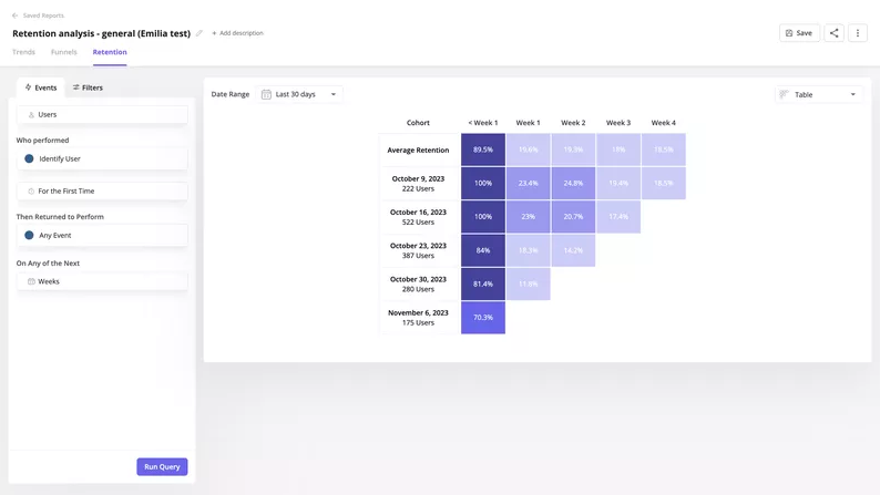
The blind spot: Cohort tables require sufficient data to produce meaningful numbers. A cohort of 12 users that retains 9 in week two reads as 75% retention, but that number is statistically unreliable at that sample size. When cohorts are small (under 30 to 50 users), retention percentages will fluctuate for reasons unrelated to anything you changed in the product.

Dot data analytics charts

Dot charts place individual data points on a scale without any aggregation. Unlike bar charts that summarize each category into a single representative value, dot charts preserve the raw data, making it possible to see individual variation, spot outliers, and understand how data values are distributed within a dataset. That precision is their main advantage over higher-level summary charts.

Dot chart types

• Basic dot chart: Each data point appears as an individual dot plotted along a scale. Clean and precise for small-to-medium datasets where you want to see every data value without losing individual data points in an average.
• Cleveland dot chart: Uses horizontal positioning along a shared axis to make comparing specific values across categories easier than a bar chart. The visual emphasis is on position rather than bar length, which works better for precise comparisons between many categories at once.
• Wilkinson chart (quantile dot chart): Stacks dots to represent point density. A column of stacked dots represents a cluster of values in the same range, making it useful for larger datasets where you want to visualize distribution shape without losing the granularity of individual data points.

When to use dot charts

Dot charts are a strong choice for analysis where precision matters and the dataset is small enough that individual points can be seen clearly. They’re effective for identifying patterns within segments, spotting outliers, and showing distributions that a bar chart or line chart would flatten into a misleading average.

Dot chart example

One way to use dot charts is to track feature interactions among active users and see, for instance, the popularity of each feature according to the number of interactions it has from users.

This way, you can see which features are mostly used by loyal customers and try to replicate their behavior in the rest of your user base to drive customer loyalty.

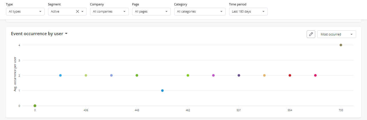
The blind spot: Dense datasets cause overplotting, where dots stack on top of each other and the chart becomes unreadable because you lose sight of individual data points. Histograms (which bucket continuous data into ranges to show distribution shape) handle large datasets better than dot charts in these situations, and density plots provide an even smoother representation of data distribution when the dataset is very large.

Bubble data analytics charts

Bubble charts extend the scatter plot format by adding a third dimension: bubble size. Each data point appears as a circle whose position on the X and Y axes represents two numeric variables, while the size of the circle encodes a third variable. This makes bubble charts one of the few chart types that can surface relationships among three numeric variables in a single, two-dimensional view.

Bubble chart types

• Scatter plot bubble chart: The most common format, where X and Y axes encode two continuous variables and bubble size encodes the third value. Works well for exploring complex datasets where multiple variables may be correlated, and for identifying outliers that stand out across all three dimensions at once.
• 3D bubble chart: Adds depth perspective to represent a fourth dimension, though this almost always reduces readability rather than improving it, and most analysts avoid 3D chart formats for this reason.

When to use bubble charts

Bubble charts are appropriate when you need to show relationships among three numeric variables in a single chart. A typical product use case: plotting feature requests on a grid where the X axis is user demand, the Y axis is estimated development effort, and the bubble size represents the potential revenue impact of shipping that feature. That single view replaces what would otherwise require cross-referencing three separate columns in a spreadsheet of feature requests.

Bubble chart example

A great instance of a bubble chart use case is for studies that require statistical depth. The following example by HubSpot shows how the gender and age of a user can have an effect on their time spent online.

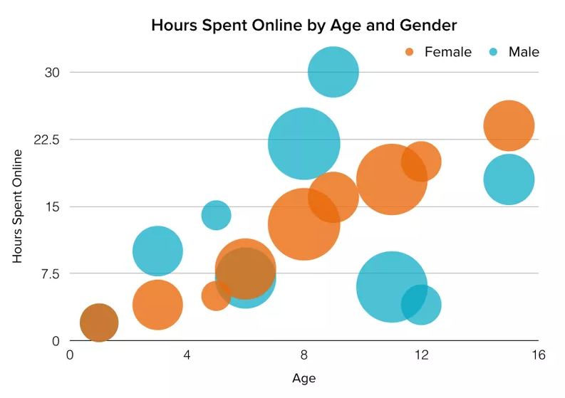
The blind spot: Humans are poor at judging area. A bubble that is twice the area of another looks only slightly larger to most viewers, which means the third variable gets systematically underestimated. Always label bubbles with their numerical values.

Stacked area data analytics charts

A stacked area chart layers multiple data series on top of each other, filling the space beneath each line to show how individual segments contribute to a cumulative total over time. Where a line chart shows each series as a separate trend, a stacked area chart displays how those series add together, making it possible to read both the overall total and the composition in a single view. The filled area beneath each line is what makes the cumulative volume visible rather than just the trend direction.

Stacked area chart types

• Basic stacked area chart: Each series is layered on top of the others, with the top edge of the chart representing the cumulative total of all series at any given point in time. Best for showing both how segments contribute and how the overall total changes.
• 100% stacked area chart: Normalizes the data so the chart always sums to 100%, which makes it easier to compare the relative proportion of each category at any point in time rather than the absolute values. Useful when the composition matters more than the total volume.

When to use stacked area charts

Stacked area charts work well when you need to show both an overall trend and the composition of that trend simultaneously. Tracking cumulative feature engagement broken down by plan type, or monitoring total active users split by geographic region over time, are both natural fits. The format is weaker when any of the individual segments are the primary story, because stacking makes them harder to read in isolation.

Stacked area chart example

An example of how to use stacked area data analytics charts is to observe the cumulative effect of users with different plans on their engagement with a specific activity and track it over time.

This way, despite seeing the same number of engagements in the last few days, you can discern if the majority of it is coming from freemium or paid users (and if it has changed recently).

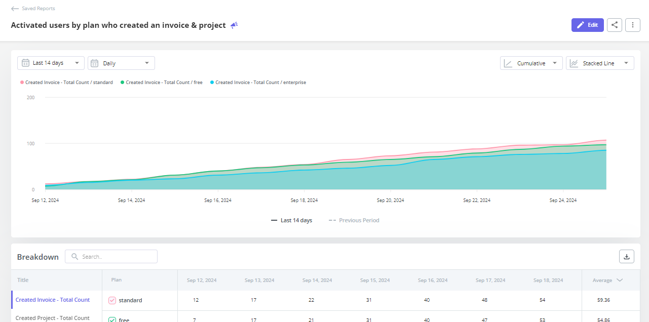
The blind spot: The bottom and top layers of a stacked area chart are easy to read; the middle layers aren’t. Any trend in a middle segment is hidden by the layers stacked above it, which means meaningful shifts in a mid-tier user segment can disappear entirely into the chart. When a specific middle segment is the focus of the analysis, use a separate line chart for that segment instead.

How to choose the right type of charts and graphs

The most common mistake product teams make with data visualization is starting with a chart type and then finding data to put in it. The right direction is the opposite: start with the question you’re trying to answer, and then pick the format that makes the answer most obvious to the person who needs to act on it.

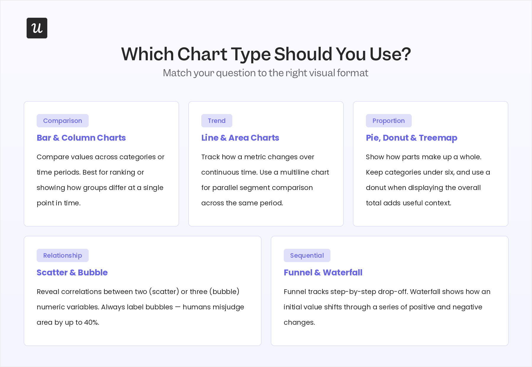
Here are the four questions you should ask to choose the chart type:

1. What decision are you trying to make? Every chart should exist to support a specific decision, not a general topic: “showing engagement” is a topic, while “deciding whether to add a second onboarding email” is a decision. The decision determines what comparison needs to be visible, which determines the chart type.

2. What type of data do you have? The structure and type of data constrain your chart options. Knowing which chart type fits which data structure is the fastest shortcut to picking the right format without second-guessing.

3. Who’s reading this? A chart that makes complete sense to an analyst may confuse a customer success manager or an executive. Simpler chart types communicate faster to mixed audiences. When in doubt, a bar chart is almost always more readable than a bubble chart, even if the bubble chart theoretically contains more information.

4. What do you want viewers to do next? If you’re trying to communicate a specific recommendation, fewer data series and more direct annotation work better than a complex chart requiring interpretation. If you’re doing exploratory analysis to discover what’s happening rather than confirm a known finding, more dimensional charts like scatter plots, cohort tables, or dot charts give you the surface area to find patterns you weren’t looking for.

A few other best practices to keep in mind:

• Keep color use consistent and minimal.
• Label your axes clearly.
• Avoid 3D effects on 2D data as they distort visual comparisons.

Impact of AI agents on data analytics charts

Most guides on chart types end at the format level. In 2026, there’s a more important question worth spending time on: are the charts you’re reading accurate?

The answer increasingly depends on what share of your product traffic is AI agents rather than human users. For many SaaS teams, that share is growing fast.

The AI agent blind spot in your charts

AI agents interact with SaaS products through APIs and MCP integrations. They execute tasks programmatically without clicking, scrolling, hovering, or opening browser sessions, which means they’re invisible to most product analytics tools.

When agents start showing up in your product, your charts read a mixed population and report it as a uniform one. Heatmaps show only human clicks; funnels count agent API completions as drop-offs; cohort tables mark agent-heavy accounts as disengaged. The accounts are active; the charts can’t see them.

The consequences are specific and largely invisible. A funnel chart might show a 30% drop-off at step 3, but if 20% of your traffic is agents completing tasks through API rather than UI navigation, that drop-off number is partially fictional. A heatmap shows no signal from agent traffic regardless of how actively those agents use the feature.

The teams getting ahead of this are rethinking what they measure for agent traffic: task completion rate, prompt volume, and account-level outcome quality rather than session metrics and click patterns. You need to view both human and agentic traffic separately.

AI agents simplify chart access

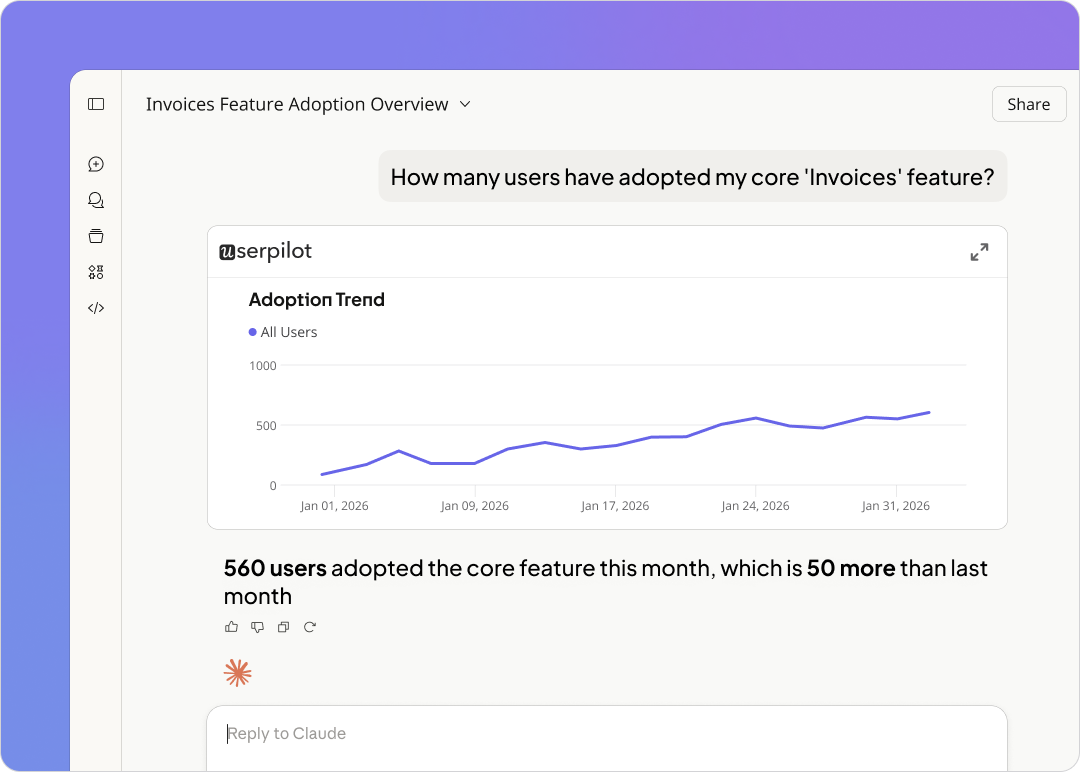
The other side of this story is more immediately useful. While AI agents create new measurement challenges in your charts, they also make your existing charts dramatically faster to access. You don’t need to navigate to a dashboard to pull a funnel analysis or check a retention cohort when you can ask for it in natural language.

Yazan Sehwail, CEO of Userpilot, described the shift directly when discussing the Userpilot MCP Server:

“If you as a marketer wanted to see, using session replay, NPS data, survey data, and product usage data, you’re able to get your answer without having to go to Userpilot, without having to pull data and upload it to someone. So this is why MCP is gonna be a game changer.”

Lia, Userpilot’s AI agent, works on the same principle. You ask Lia a question in plain language, and Lia surfaces the relevant chart and can keep monitoring your metrics automatically.

See your product data in one place with Userpilot

The ten data analytics chart types covered here, from bar charts for category comparison to cohort tables for retention tracking, are available natively in Userpilot’s analytics platform alongside the tools to act on what they show. When a funnel chart reveals a drop-off, you can build a tooltip or checklist to address it in the same platform. When a cohort table shows a segment disengaging, you can trigger a targeted in-app flow for that group immediately.

Get a 14-day free trial for Userpilot now to start analyzing your SaaS product’s performance.